One of the many great things about Microsoft Excel is that it allows you to manipulate large amount of data to make better, calculated business decisions. In the previous posts, we saw how we can create how we can use Data Tables, create Outlines, use Formulas, etc. in Excel. In this post, let us look at PivotTables.
A PivotTable in Microsoft Excel allows you to summarize large amounts of data from any range of tables that has labels for each columns. PivotTables are one of the easiest way to summarize, analyze, explore and present large amount of data with a few clicks!
Few Important Things to Note:
- Ensure that your Excel Worksheet data is organized in a tabular format without any blank rows or columns.
- Using Excel Tables as a PivotTable source is one of the easiest, because, in case you wish to modify the source table, your PivotTable automatically gets updated accordingly.
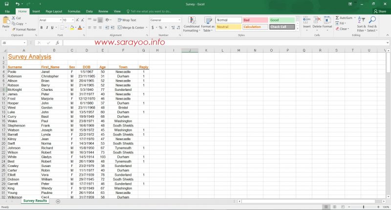
- Data type in your columns must be the same. For example, if your column name is “Age” which has the data type as number, ensure that all the data in that column is a number.
How to Create a PivotTable in Excel 2016
Step 1: Open your Excel Worksheet, ensure that your Worksheet meets the above mentioned items under ‘Important Things to Note’ (1 to 3).
Step 2: To create a PivotTable for your Excel Worksheet, click on Insert Tab >> and then click on PivotTable >> Select the Table / Range of cells you want to create the PivotTable for >> Select where you like the PivotTable to be created – either on the same Worksheet or on another Worksheet in the same Excel Workbook.
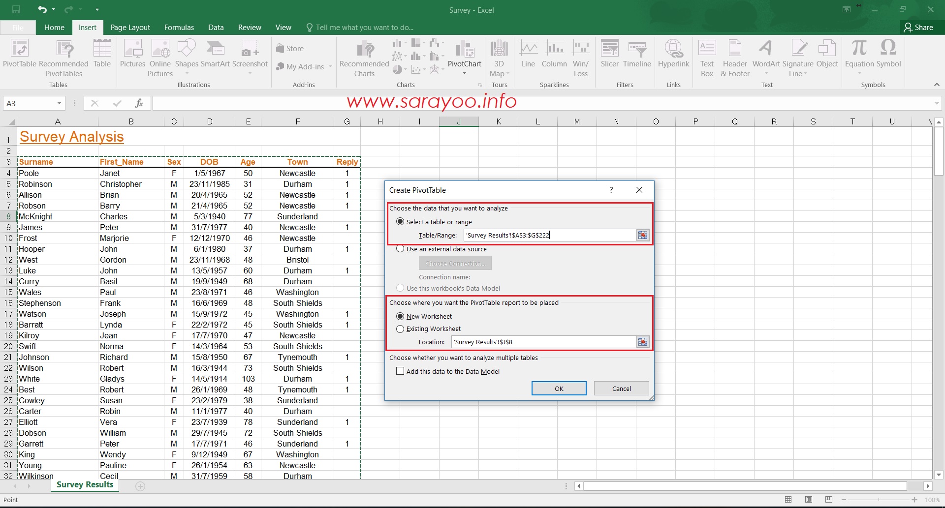
Once you do that, you have a PivotTable created in the Workbook according to your selection – either on the same Worksheet or on a new Worksheet, like how I did here.
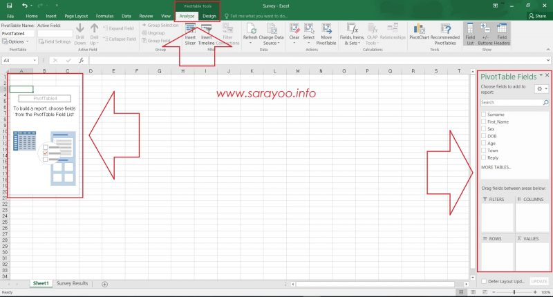
As you can see, there are two new Tabs appearing at the top menu – Analyze and Design under the PivotTable and a blank PivotTable and a set of PivotTable field list on the right hand side of your window.
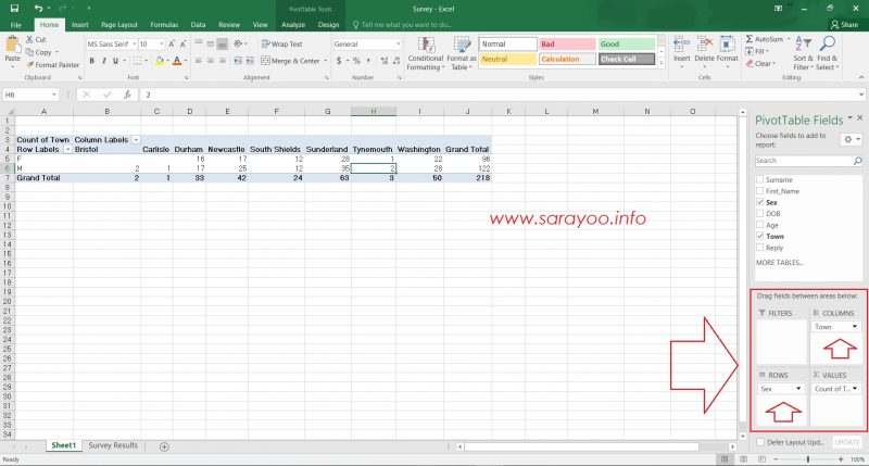
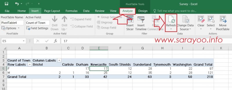
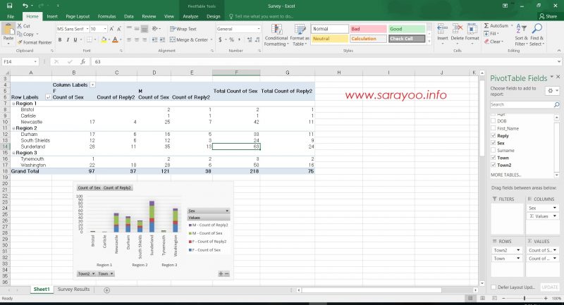
Step 3: You can drag and drop the PivotTable fields to the PivotTable areas according to your requirements. In this example, I’m going to drag “Sex” field in the Columns area and “Town” field in the Rows area and drag the “Town” field again in the ∑ Values area (Count of Town) as shown below:

A PivotTable is created as shown in the image above which shows the count of people surveyed, divided into their Sex (Male / Female) and organized by town.
NOTE: When you click away from the PivotTable, the PivotTable Field List is hidden. So, in case, if you don’t see the PivotTable Field List, click on the PivotTable!
If you want to organize the PivotTable differently, you can re-arrange the Fields in the PivotTable Field List as you want. For example, if you interchange the field “Sex” and “Town” to Rows area and Columns area respectively, you will get a PivotTable as shown below:
If you make changes to your Excel Worksheet table, you need to go to the PivotTable >> Analyze tab >> Click Refresh button under the Data Group for the PivotTable to be updated.
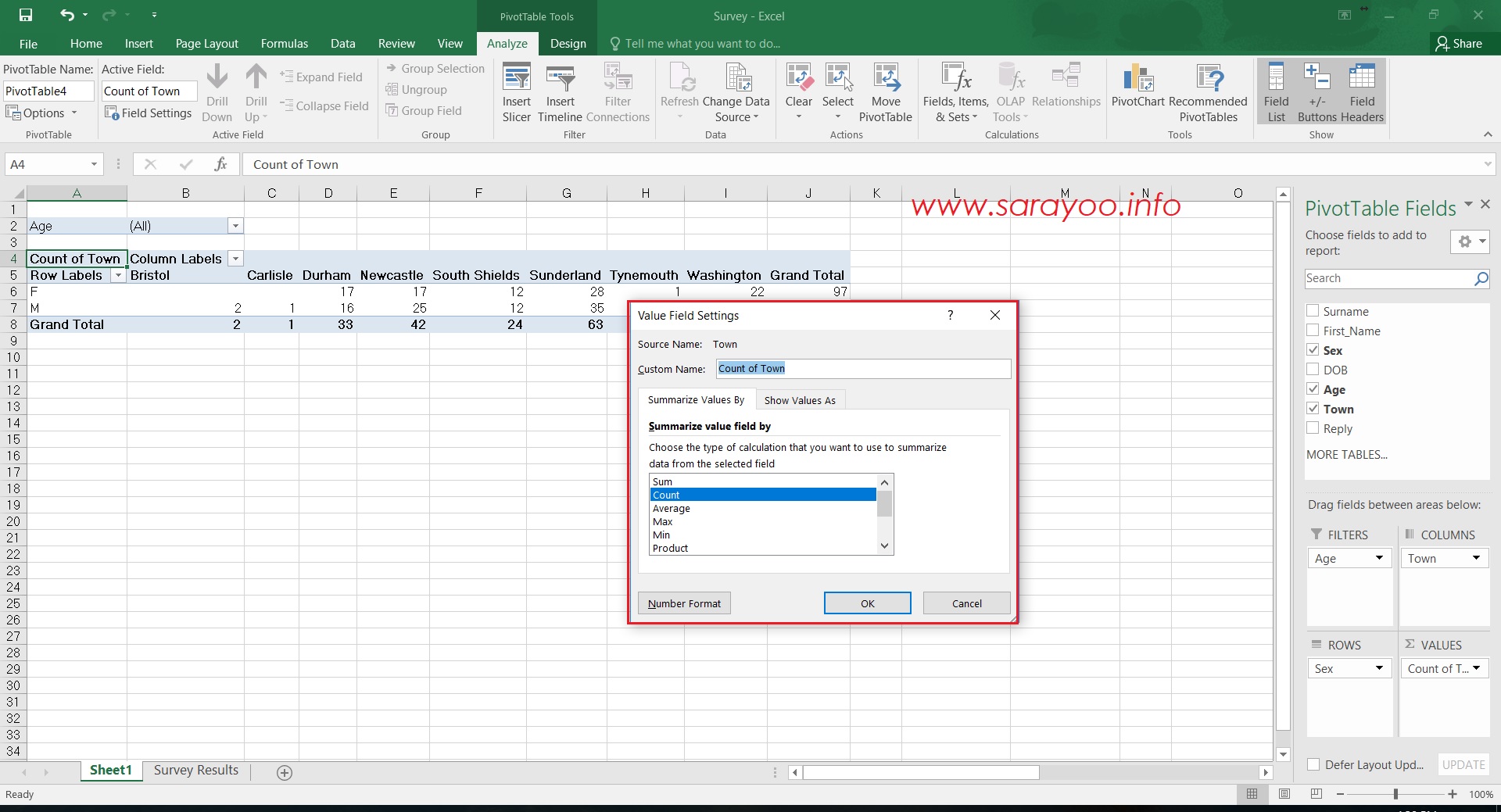
Summarize Values by
PivotTable values which are places in the Value area is displayed as a “SUM” by default. If the data type is Text, Excel automatically display it as “COUNT” (in our example, Count of Town). However, you can change this default calculation by clicking on the arrow to the right of the field name >> then select “Value Field Settings” option as shown below:

Filtering a PivotTable in Excel 2016
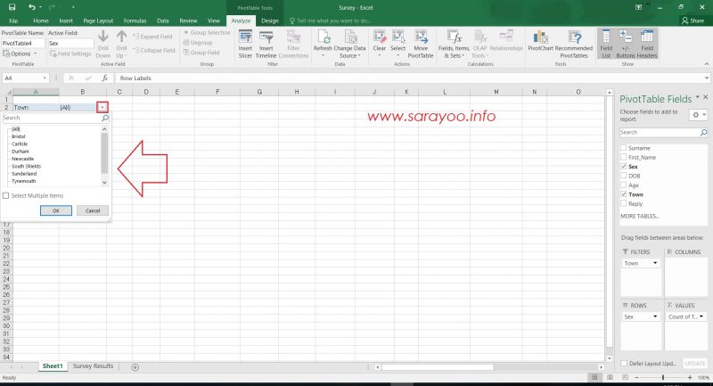
PivotTable can be filtered using the fields from the PivotTable Field list. A single data can be displayed by simply dragging a field from the Field List to the Report Filter area. This can then be controlled by using the drop down list and selecting what is required to be shown.
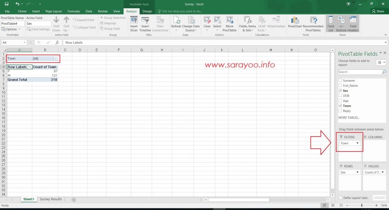
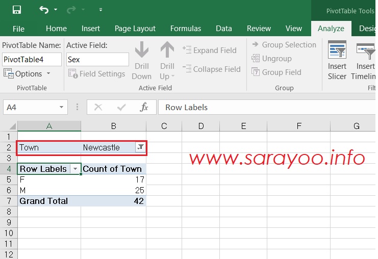
You can select whichever the Data you want to filter by, as shown below. For example, if you select Town as ‘Newcastle’, it filters the data only for Newcastle and display in the PivotTable.
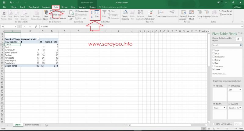
Grouping and Sorting in PivotTables
In addition to summarizing and filtering PivotTable data, we can also arrange and analyze data in a PivotTable by grouping them according to various categories.
In our example survey, we can summarize all data by month and it can be further grouped by Quarter 1, Quarter 2, etc. or grouped by Town as Region 1, Region 2, etc.
You can select multiple items by pressing CTRL Key. Once after making your selections, click on Analyze Tab >> Group Selection. You can then select the Group name and change the name to whatever the name you wish to give to that group.
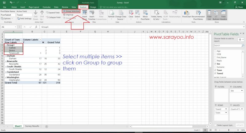
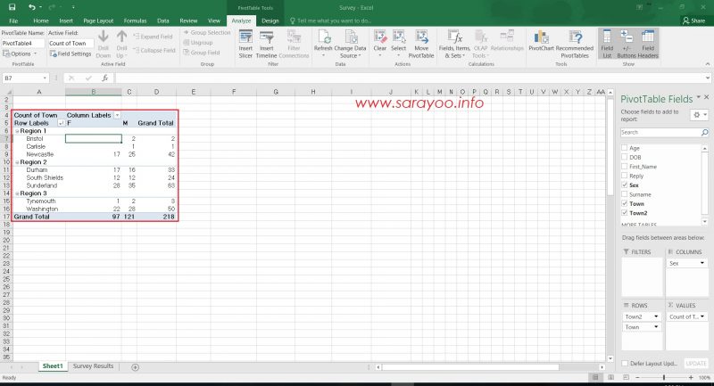
You can also collapse or expand each group by clicking on the + and – signs appearing along each group.
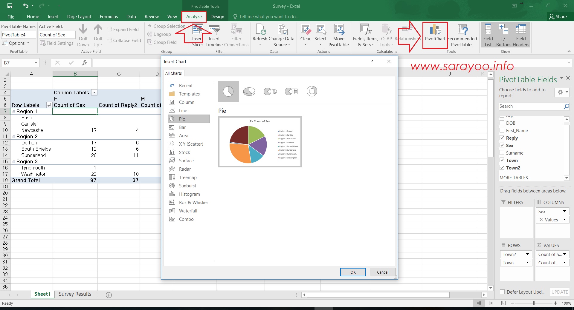
Creating a PivotTable Chart / Pivot Chart
You can easily create a PivotTable chart in few clicks using Excel 2016. Once after you create your PivotTable, click on the Analyze Tab >> then click on PivotChart >> then decide which chart you would like to create from the popup menu.
Delete a PivotTable
If you no longer want to use the PivotTable you created, you can simply delete it by selecting the entire PivotTable, and click Delete on your Keyboard. Deleting a PivotTable won’t affect any of the data in your Worksheet.
Hope these tips help you! You can follow me on Twitter @sarayoo.info or Google+ or Like me on my Facebook or on my LinkedIn for more updates, technology tips and tricks etc. Please leave your comments in the comment section or contact me if you have any other questions.